Newsletter Volume 11, Issue 1 March 2026
SBTn assessment in Laminated Soil Systems based on DEM Simulation of CPT
School of Engineering and Technology, the University of New South
School of Engineering and Technology, the University of New South
Abstract
Cone penetration testing (CPT) has been widely used for soil stratigraphy and geotechnical property determination. However, in laminated soil systems, the performance of the widely used updated soil behaviour type (SBTn) method for soil classification remains uncertain. This study checks the effectiveness of SBTn in the multi-thin layers interbedded soil system. Numerical simulations of CPT reveal that it is unfeasible to distinguish laminated layer(s) (1Dcone) by CPT as the profile shows weak transitions and appears as a single layer. The SBTn method tends to predict the silt interlayer boundaries deeper than their true positions, but shallower for clay boundaries. Such boundary identification becomes harder in weak-soil-dominated systems.
Keywords: laminated soil systems; DEM simulation; CPT; Soil Behaviour Type
1. Introduction
Cone penetration testing (CPT) is a reliable method for in situ soil testing, providing continuous data (cone tip resistance qc, cone shaft resistance fs) to evaluate critical geotechnical design parameters, soil stratigraphy, pile capacity, and liquefaction potential. To establish the soil model for design or research purposes, the CPT profile is normally used to generate soil stratigraphy at first and then to predict property parameters of each layer based on proper correlations, especially for situations that lack borehole or laboratory test information.
The SBT and SBTn (soil behavior type) charts, introduced by Robertson (1990, 2009), are effective for homogeneous or thickly layered soils (Ku et al., 2010). But in laminated soil systems (i.e., sand profiles with thin interbedded silt or clay layers, which are common in environments like deltas or alluvial plains), qc and the derived SBT index (Ic) often represent a mixed response from neighboring layers, leading to misclassification and inaccurate soil property estimates. Therefore, it is necessary to understand the interacting mechanism between the cone and soils during the penetration process in the laminated soil system.
This study performs a series of numerical simulations of the cone penetration tests in laminated soil systems by discrete element method 3D (PFC3D 7.0) and aims to verify the performance of SBTn in complex soil systems (thin silt/clay layer(s) interbedded in sand). Meanwhile, by observing the cone penetration process from micro perspective in multi-thin layered situations, the mechanism of interaction between different layers and the cone can be described.
2. Numerical model simulation and calibration
2.1 Numerical model and material parameters
A three-dimensional Particle Flow Code, PFC3D 7.0, was used to numerically simulate both Cone Penetration Tests and Triaxial tests.
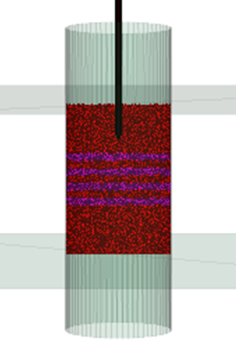
The CPT model consists of a chamber (cylinder, 0.7 m in diameter, 1m in length), a cone (0.044 m in diameter, 0.16 m sleeve length, apex angle of 60°), and K0 boundary conditions (a constant pressure of 100 kPa applied at the top and bottom, with a constant radial confining pressure of 50 kPa). The cone was pre-embedded 0.2 m into the soil sample, and the total penetration depth was 0.5m. as shown in Fig. 1 (a & b). The penetration rate of the cone is 0.05 m/s. The inertial number under this penetration velocity is 1.0*10-3, satisfying the requirement for a quasi-static condition as suggested by Janda and Ooi (2016).
 |
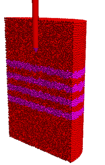 |
| (a) | (b) |
| Fig. 1. Diagram of Cone Penetration Test in a multilayered soil system | |
Three types of soil were used in the model. The minimum, median, and maximum particle sizes of the three kinds of soils used in the model are dmin = 0.0124 m, d50 = 0.0143 m, and dmax = 0.0164 m, respectively. The inter-particle properties used to simulate soils are summarized in Table 1. The parameters were calibrated using laboratory triaxial tests of Ottawa sand (Khosravi et al. (2020); Su et al., (2019); and Su, (2019)) and a silt (Pietruszczak et al. (2003). The friction coefficient between the particles and pile / chamber (wall) is 0.2 and 0.1, respectively.
Table 1. Soil parameters for DEM modelling
| Soil/ Object Parameters | Sand | Silt |
| Contact model | Rolling resist linear | Rolling resist linear |
| Particle size (D50) (mm) | 0.0143 | 0.0143 |
| Particle density (ρs) ( kg/m3) | 2650 | 2650 |
| Initial porosity | 0.367 | 0.375 |
| Porosity after consolidation | 0.38 | 0.389 |
| Particle normal stiffness (kn) (N/m) | 5.00E+06 | 4.00E+05 |
| Particle shear stiffness (ks) (N/m) | 2.50E+06 | 2.00E+06 |
| Inter-particle friction coefficient | 0.35 | 0.28 |
| Damp ratio | 0.7 | 0.7 |
| Special parameters used by particular models |
rr_fric: 0.4 | rr_fric: 0.38 |
2.2 Numerical modelling series
A total of 15 soil samples were simulated as summarized in Table 2. There are three cases of homogeneous soil samples (sand, silt and clay) and two types of laminated soil cases: sand-silt (Tests 4 to 9) and sand-clay (Tests 10 to 15). Each laminated soil case involves two arrangements: thin weak/soft layers (silt/clay) interbedded in sand (Tests 4 to 7 and Tests 10 to 13), or strong/stiff sand layers interbedded in soft silt/clays (Tests 8, 9, 14 and 15). Different numbers of interlayers were considered, ranging from 1 to 4. The thickness of the interlayers and the spacing between them is 0.05m, which is near one diameter of CPT cone (Dcone=0.044m). The primary variable in evaluating the influence of weak layer(s) on the multi-layer soil system is the proportion of soft/weak soil relative to the entire soil sample (the ratio between weak/soft soil layer thickness and total sample thickness, Rt).
Table 2. Summary of the simulations
| Soil System | Test No. | No. of Thin Layers | Weak Soil Proportion (Rt) |
| Sand | 1 | – | 0% |
| Silt | 2 | – | 100% |
| Sand with thin silt layers | 3, 4 | 1, 2 | 10%, 20% |
3. Results
3.1 Macro behaviour
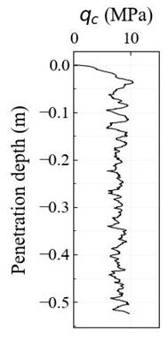
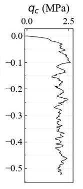
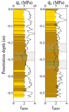
Fig.2 illustrates the variations in CPT measurements (qc, fs, and Rf) with depth in a single to multiple thin weak layers (silt/clay). The corresponding soil categorization using the SBTn method are also shown in colors. The locations of the weak layers are marked in the light grey shaded area. For the CPT readings, the single thin weak layer produces a distinct transition zone, but within the multi weak layers the qc profiles show no clear transitions, making the deposit appear as a single layer.
 |
 |
 |
|---|---|---|
 |
||
| Fig. 2. CPT profile in sand, silt and sand with one or two layers of silt. | ||
3.2 Micro analysis
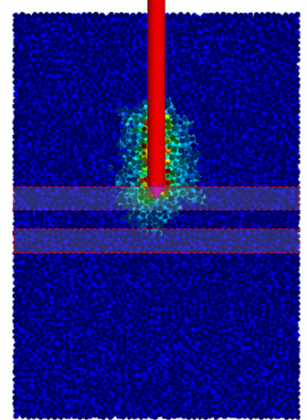
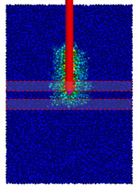
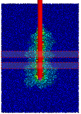
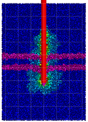
To examine how the inter-soft layers influence the CPT profiles, Fig. 3 shows the soil particle movements during the penetration process of the cone into the sand with two layers of silt. Fig. 3 (a) to (c) illustrates the movements of sand particles at the penetration depths of 0.225 m, 0.275 m, 0.475 m. These depths correspond to the cone tip entering the first silt layer and the middle sand layer, and about 2dc through the second silt layer. Fig. 5 (d) demonstrates the deformation of the interbedded layers at 0.475 m penetration depth.
Fig. 3 (d) shows that the interfaces of the interbedded layers deflect, and sand/ silt particles get into the silt / sand layer with the cone during penetration, which is consistent with the laboratory results described in Van Der Linden (2018). This distortion of the interface results in the cone tip being surrounded by particles from the upper layer rather than the lower layer when it reaches the soil layer interfaces. As a consequence, the qc value at the interface still reflects the properties of the upper layer soil. This partially explains the difficulty in distinguishing the layer boundaries using qc values. As the top interface has the largest deflection, more upper sand particles get into the silt layer. This explains the poor performance of using qc to determine the top boundary of the layered zone. As a result of the distorted silt layer, SBTn method predicted a deeper top interlayer boundary. This finding is further verified in Fig. 6.
 |
 |
 |
 |
 |
| (a) | (b) | (c) | (d) | |
| Fig. 3. Displacement fields of two silt layers interbedded in sand when the penetration depth is: (a) 0.225m; (b) 0.275m; (c) 0.475m; (d) 0.475m |
||||
4. Discussion & Conclusions
This study uses PFC3D 7.0 to simulate cone penetration tests in laminated soil systems, with the aim of evaluating the soil boundary identification method based on CPT measurements (SBTₙ method by Robertson (2009)). This study reveals that layering identification by SBTn faces challenges in predicting both the soil layering and soil type in multi-thin-layered soil system. Meanwhile, for incohesive soil system, SBTn tends to predict a deeper top boundary of the laminated area. The findings indicate that the driven behavior of press-in piles in soils with multi-layer laminated soil systems can be difficult to predict using the current CPT profile, which requires further study.
References
Janda, A., & Ooi, J. Y. (2016). DEM modeling of cone penetration and unconfined compression in cohesive solids. Powder Technology, 293, 60-68.https://doi.org/10.1016/j.powtec.2015.05.034
Khosravi, A., Martinez, A., & DeJong, J. T. (2020). Discrete element model (DEM) simulations of cone penetration test (CPT) measurements and soil classification. Canadian Geotechnical Journal, 57(9), 1369-1387.https://doi.org/10.1139/cgj-2019-0512
Ku, C. S., Juang, C. H., & Ou, C. Y. (2010). Reliability of CPT I c as an index for mechanical behaviour classification of soils. Géotechnique, 60(11), 861-875. https://doi.org/10.1680/geot.09.P.097
Pietruszczak, S., Pande, G. N., & Oulapour, M. (2003). A hypothesis for mitigation of risk of liquefaction. Geotechnique, 53(9), 833-838. https://doi.org/10.1680/geot.2003.53.9.833
Robertson, P. K. (1990). Soil classification using the cone penetration test. Canadian Geotechnical Journal, 27(1), 151-158. https://doi.org/10.1139/t90-014
Robertson, P. K. (2009). Interpretation of cone penetration tests – a unified approach. Canadian Geotechnical Journal, 46(11), 1337–1355. https://doi.org/10.1139/T09-065
| << Previous | Newsletter Top | Next >> |